My Journey Learning AI for Songwriting: LSTMs and Taylor Swift

I spent last 4 months learning with the Machine Learning Zoomcamp. When it was time for the final project, I wanted to try something new that wasn’t covered in our sessions. Then, I heard all the hype about Taylor Swift’s tour and thought, ‘Why not try creating lyrics in her style?’

So here’s a little story about my adventure with LSTM models, trying to generate songs. You can peek at my project here: Project Taylor Swift Lyrics Generation.

Project Overview

My mission was to capture the style of Taylor Swift’s songs, which meant I first needed to get my hands on her lyrics. A quick Google search for ‘Taylor Swift lyrics dataset’ led me to a useful dataset on Kaggle, but there was a catch: it only covered 6 of her albums, and she’s released 10. To fill in the gaps, I used the Genius API to scrape the missing lyrics, making sure I had a complete set to work with.

If you’re curious about how I managed the scrapping part, you can check out my code here. It’s where I laid out the steps I took to gather all those lyrics. Using this code you can create your own dataset of lyrics for any artist. And as for the dataset I compiled, which now includes lyrics from all 10 albums, you can find it here.

Let’s take a closer look at the data. We’ve got albums and tracks, organized with the lyrics broken down line by line.

The data has 4862 rows and 7 columns. And if we look at the summary table, it shows we’ve got all 10 albums in there.

If you try to research the topic of AI songwriting, the first thing that the Internet will offer you are LSTM models.

Quick Introduction to LSTM

LSTMs are a type of recurrent neural network (RNN) that are really good at remembering things for a long time. They’re perfect for when you’re dealing with sequences, like text or anything that changes over time.

Here’s the core idea of how they operate:

• Cell State: This is the LSTM’s memory track, carrying information all the way through the sequence. It holds on to the important bits and gets rid of the stuff we don’t need.
• Gates: Filters that decide what information should be kept or thrown away at each step in the sequence.

Inside an LSTM, we have:

1. A Forget Gate that decides what to forget from the past information.
2. An Input Gate that chooses which new information to add.
3. An Output Gate that determines what the next output should be, based on the updated information.

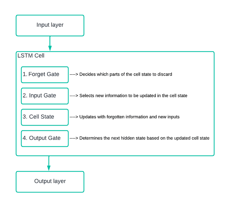
LSTMs are a step up from traditional RNNs (Recurrent Neural Networks) because they’re much better at remembering things for a long time. RNNs struggle with this because they tend to forget the older information as new data comes in. LSTM keeps track of what’s important and ignore what’s not, making it really smart at handling data that changes over time.

Alongside LSTMs, I was also looking into GRUs (Gated Recurrent Units), which are kind of like LSTMs’ younger sibling. They’re simpler because they have fewer gates, making them faster to work with but not always as nuanced in handling memory as LSTMs.

Word vs. Character

In AI and with things like LSTM models, what we consider as the smallest piece of text — a word or a character — really matters. It’s about whether we look at each word as a whole or break things down to letters and punctuation.

Word-Level Approach

Word-level method focuses on each word in a sentence, treating them as unique items. Model trained this way learns from loads of data, understanding and predicting text word by word. This is great for getting the hang of the overall meaning and keeping things readable since the model is less likely to spit out random words. But, there’s a catch: the model’s vocabulary is only as good as what it’s been trained on. Throw in a rare word, and it might get stumped. Plus, remembering a whole dictionary’s worth of words isn’t easy — it needs a lot of memory.

Character-Level Approach

Then there’s the character-level approach, where everything gets broken down to the bare bones — letters, digits, punctuation, you name it. This model stitches together the next character in line, slowly forming words and sentences. It’s pretty handy when dealing with new or unique words since it constructs them letter by letter. And it doesn’t need to memorize a massive vocabulary, just the basics like the alphabet and some symbols. Though it might miss the bigger picture or the full context since it’s so focused on the tiny details. And sometimes, the sentences it comes up with can be a bit off, not quite hitting the mark on coherence or grammar.

After seeing a character-level lyrics generator on Kaggle, I decided to go with the word-level approach for my project. I hoped it would keep the perfect balance between capturing the essence of lyrics and maintaining clear, coherent text.

Data Cleaning and Preparation

Now we’ll go through the steps to prepare our data for the LSTM model. This code block below lays out the process of getting our text data into the right format for training.

When we set up data for LSTM, we usually break it down into smaller pieces. For our project, where we’re focusing on words, this means organizing the data into sequences of words. Here’s how we do it:

1. Tokenization:

• We begin with our massive collection of lyrics. We combine the lyrics from every single row into one long text string. Next, you’ll see an example of these combined lyrics:

combined_lyrics: he said the way my blue eyes shined 
put those georgia stars to shame that night
i said that is a lie
just a boy in a chevy truck
that had a tendency of gettin' stuck

• After we have our long text string, we break it down into individual words. This step is known as tokenization, where every word in our dataset gets identified and separated out. You might notice in the code, I use tokenizer.fit_on_texts([combined_lyrics]) to train the tokenizer on our combined lyrics. When you see total_words = len(tokenizer.word_index) + 1 in the code, that's figuring out how many unique words we have in our lyrics, making up the vocabulary.

2. Generating Input Sequences:

• Now we move on to creating input sequences from our text data, which, for my project, are the lines from our cleaned dataset. We use a for loop to go through each lyric line. For every line, we change the words into their number codes, based on our vocabulary. Then, inside this loop, there’s another loop that makes n-gram sequences out of these number codes. So, we’re building up sequences of different lengths for each line, adding one word at a time to make a new sequence. Below, you’ll see what comes out after one run of this process:

total words:  3573
line: he said the way my blue eyes shined
token list: [47, 72, 3, 87, 11, 239, 89, 693]
n_gram_sequence: [47, 72]
n_gram_sequence: [47, 72, 3]
n_gram_sequence: [47, 72, 3, 87]
n_gram_sequence: [47, 72, 3, 87, 11]
n_gram_sequence: [47, 72, 3, 87, 11, 239]
n_gram_sequence: [47, 72, 3, 87, 11, 239, 89]
n_gram_sequence: [47, 72, 3, 87, 11, 239, 89, 693]

3. Formatting the Input:

• After we’ve got our sequences, we need to shape them so they fit what the LSTM network can handle. This often means tweaking the size and structure of our input data to match the LSTM’s needs. That’s where padding comes in — it helps us make sure every sequence is the same length, which is a must-have for LSTM since it works with fixed-length inputs.

max_sequence_len: 23
input_sequences: [[47, 72], 
                  [47, 72, 3], 
                  [47, 72, 3, 87], 
                  [47, 72, 3, 87, 11], 
                  [47, 72, 3, 87, 11, 239], 
                  [47, 72, 3, 87, 11, 239, 89], 
                  [47, 72, 3, 87, 11, 239, 89, 693],
                  [169, 300],
                  ...

• After padding, each row in our final array will consist of 23 elements, ensuring uniformity across all input sequences for the LSTM model.

input_sequences: [[   0    0    0    0    0    0    0    0    0    0    0    0    0    0
     0    0    0    0    0    0    0   47   72]
 [   0    0    0    0    0    0    0    0    0    0    0    0    0    0
     0    0    0    0    0    0   47   72    3]
 [   0    0    0    0    0    0    0    0    0    0    0    0    0    0
     0    0    0    0    0   47   72    3   87]
 [   0    0    0    0    0    0    0    0    0    0    0    0    0    0
     0    0    0    0   47   72    3   87   11]
 [   0    0    0    0    0    0    0    0    0    0    0    0    0    0
     0    0    0   47   72    3   87   11  239]
 [   0    0    0    0    0    0    0    0    0    0    0    0    0    0
     0    0   47   72    3   87   11  239   89]
 [   0    0    0    0    0    0    0    0    0    0    0    0    0    0
     0   47   72    3   87   11  239   89  693]
 [   0    0    0    0    0    0    0    0    0    0    0    0    0    0
     0    0    0    0    0    0    0  169  300]

4. Breaking Down the Sequences:

• Next, we divide our sequences into two parts: predictors and labels. The predictors include every token in a sequence except for the last one, which serves as the label.
• To make it suitable for the LSTM model, we convert these label integers into a one-hot encoded format using to_categorical(label, num_classes=total_words). One-hot encoding transforms each integer into a vector full of zeros except for the position of the integer, which is set to one. This way, every label is clearly marked in a format the model can understand.

I talked about using a ‘cleaned dataset’ earlier, which means we cleaned up the lyrics before getting into the data prep. Our original lyrics had a mix of capital letters, punctuation, and contractions which could mess things up. So, I went through and cleaned it up: turned all the letters lowercase, stripped out the punctuation, and swapped common contractions with their expanded forms. For example, I changed “ain’t” to “is not,” “aren’t” to “are not,” and so on.

"ain't": "is not", 
"aren't": "are not",
"can't": "cannot", 
"'cause": "because", 
"could've": "could have", 
...

This prep work made the text more consistent, setting a solid foundation for building our dictionary and moving forward. Check out the cleanup process in the code snippet below.

Then, of course, I also made sure to check the text for any non-ASCII characters.

non-ASCII characters ['\x85', '\x91', '\x93', '\x94', '\x96', '\x97', 'é', 'í', 'ó', 'е', '\u2005', '—', '’', '\u205f']

Since we’re dealing with lyrics, there might be some unusual words in there. Let’s take a look at what we’ve got:

That’s the sample of the output we end up with:

 'halfmoon': None,
 'friendsyou': None,
 'dreamscapes': None,
 'twentyyear': None,
 'mirrorball': None,
 'whitecollar': None,
 'afternoons': None,
 'notfunnyat': None,
 'openshut': None,
 'whoaahoh': None,
 'ladadada': None,
 'youpainted': None,
 'selfexpression': None,
 'getyouout': None,
 'coasttookher': None,
 'howdidamiddleclass': None,
 'intheshade': None,
 'thebeachesnow': None,
 'oohwoooohoohooh': None,
...

You can notice a lot of the words in the list are pretty odd, so I decided to remove them. Like any set of lyrics, ours also had some duplicate lines. Let’s take a look at those.

lyric_clean
you might also like                   62
welcome to new york                   27
all you had to do was stay            15
oh oh                                 13
look what you just made me do         13
                                      ..
and the sparks fly                     2
but you might have to wait in line     2
got that ah i mean i mean              2
and you just see right through me      2
just like all those times before       2

Removing these strange words might change the style a bit, but I didn’t want to emphasize them too much. If we do, the output might just keep repeating the same things. So, I took out the duplicated lines.

I also took a look at the most common words.

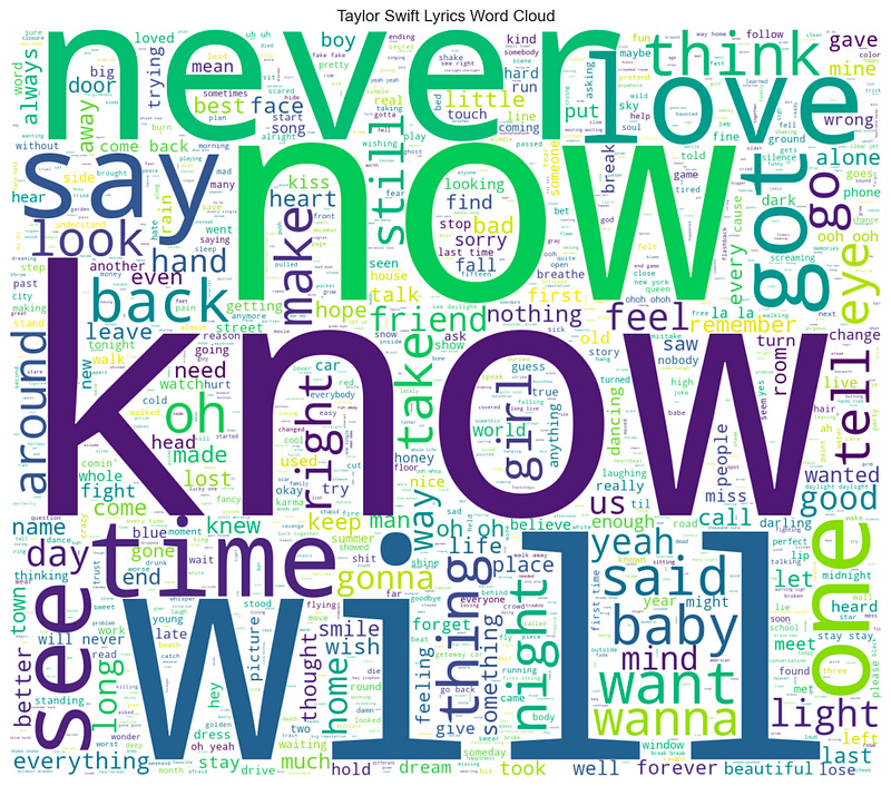
[('know', 274),
 ('will', 242),
 ('never', 203),
 ('now', 203),
 ('oh', 190),
 ('time', 166),
 ('back', 153),
 ('love', 145),
 ('see', 142),
 ('one', 141)]

I was a bit skeptical about all those “oh” words in the lyrics, but in the end, I chose to leave them as they were.

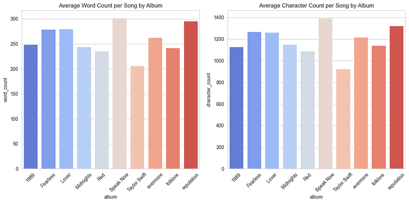
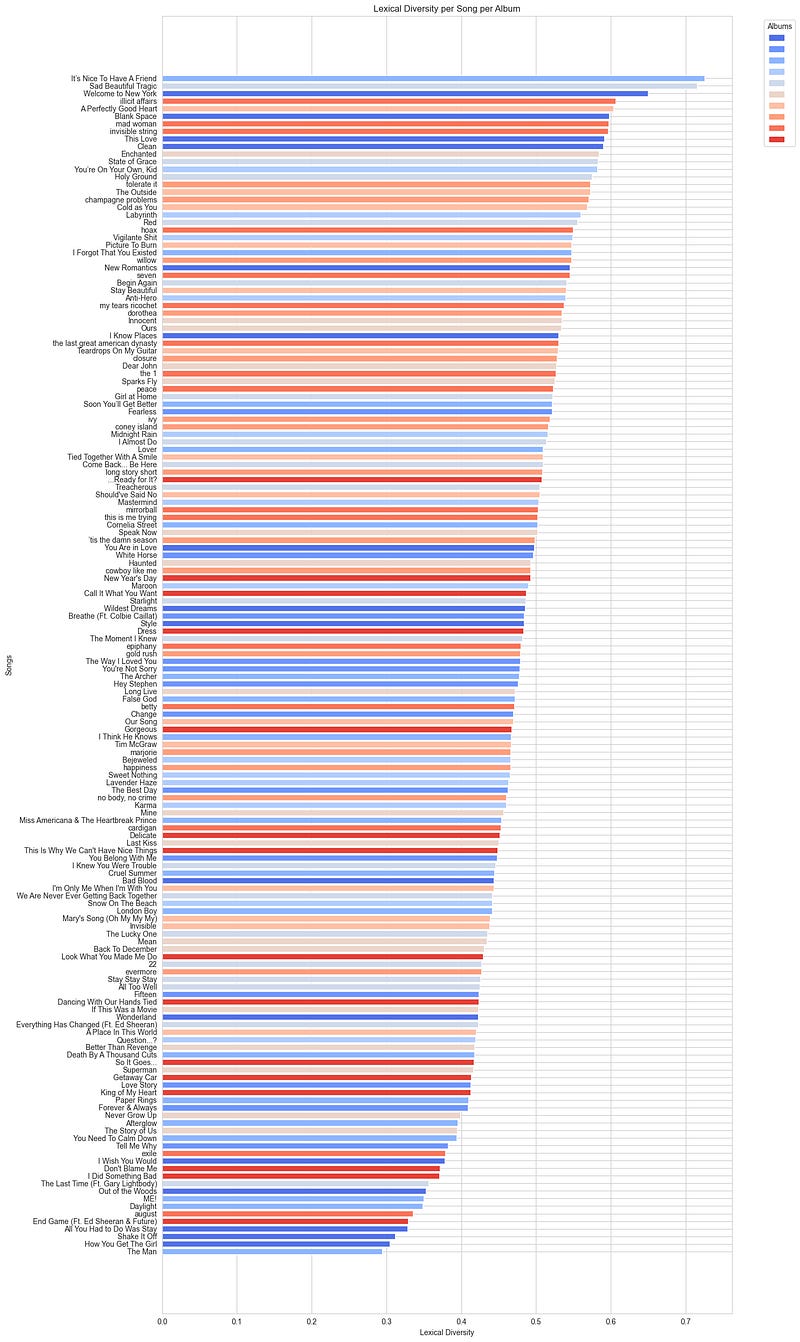
Here are a few visuals from the exploratory data analysis (EDA) — I managed to whip up some pretty neat graphs, and I’m still quite pleased with how they turned out.

The Challenge of Metrics

Now, let’s dive into the tricky part: figuring out how to measure our model success. When it comes to generating lyrics with AI, like using LSTMs, we’re in a whole different territory compared to standard machine learning tasks. It’s not like you can easily tell if you’re right or wrong.

In regular tasks, you’ve got a clear metric: accuracy. It’s all about getting the right answers, with a simple percentage telling you how many you got spot on. But with lyrics, what’s “right” isn’t so straightforward. Lyrics aren’t just about right or wrong; they’re about style, rhyme, rhythm, and the feelings they evoke. So, the usual way of measuring accuracy doesn’t really cut it for judging the quality of AI-generated lyrics.

There is another metric — perplexity is often used as a measure. Perplexity evaluates how well a probability model predicts a sample. A lower score indicates that the model is better at making predictions, as it suggests the model is less perplexed by the data. However, while perplexity can be useful for comparing models or iterations of a model, it does not necessarily correlate with the human perception of quality or creativity in the generated lyrics.

In the end, judging AI-crafted lyrics often boils down to human input. We look at things like how creative, coherent, and emotionally resonant the lyrics are, or how well they stick to a certain theme or style. But, leaning on human opinions brings its own hurdles, such as inconsistency and bias. Different people might see the same set of lyrics in entirely different lights based on their personal tastes and what they value in music, which can lead to varied assessments.

Doing this project solo was a bit of a blessing since I didn’t run into any debates with myself. I continued to rely on accuracy and perplexity as my metrics, but ultimately, the final judgment on quality rested with me.

I chose to experiment with a few different setups: a standard LSTM, an LSTM wrapped in bidirectional layers, and a GRU, to see how they stack up. And for desert — initialize my embedding layer with the weights from our GloVe embedding matrix.

Model 1

• Input Layer (Embedding Layer): This layer transforms our input data into dense vectors of a fixed size (100-dimensional vector). The layer is set to handle sequences that are 22 words long, which is max_sequence_len-1 in our case.
• LSTM Layer (150 units): Here, we have 150 LSTM units working to understand the sequence and context of our words.
• Dropout Layer (0.1 dropout rate): This layer randomly skips some neurons during training, a trick to avoid overfitting by making the model less sensitive to the specific weights of neurons.
• Output Layer (Dense Layer): The final layer has as many neurons as there are unique words in our vocabulary, setting the stage for the model to choose the next word.

For the loss function, we’re using categorical_crossentropy because we're dealing with a multi-class classification (each word prediction is a class). Plus, I've implemented early stopping (val_loss) to prevent over-training by halting the training process if the model's performance stops improving.

Let’s take a closer look at how the model was trained and the metrics that came out of it. We’ve got some outputs and graphs to show how things went down during the training process, giving us insights into the model’s performance and learning progress.

Total params: 1047423 (4.00 MB)
Trainable params: 1047423 (4.00 MB)
Non-trainable params: 0 (0.00 Byte)
_________________________________________________________________
Epoch 1/100
882/882 [==============================] - ETA: 0s - loss: 6.0899 - accuracy: 0.0498 - perplexity: 441.39474756818714
882/882 [==============================] - 16s 15ms/step - loss: 6.0899 - accuracy: 0.0498 - val_loss: 5.8455 - val_accuracy: 0.0723
Epoch 2/100
882/882 [==============================] - ETA: 0s - loss: 5.4689 - accuracy: 0.1038 - perplexity: 237.2067566601589
882/882 [==============================] - 8s 9ms/step - loss: 5.4689 - accuracy: 0.1038 - val_loss: 5.4887 - val_accuracy: 0.1256
Epoch 3/100
880/882 [============================>.] - ETA: 0s - loss: 5.0650 - accuracy: 0.1371 - perplexity: 158.42614834644223
...
882/882 [==============================] - ETA: 0s - loss: 3.5529 - accuracy: 0.2713Restoring model weights from the end of the best epoch: 6.
 - perplexity: 34.91468334300078
882/882 [==============================] - 7s 8ms/step - loss: 3.5529 - accuracy: 0.2713 - val_loss: 5.3372 - val_accuracy: 0.1893
Epoch 9: early stopping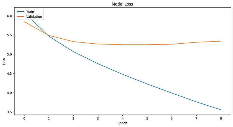

The training stopped at epoch 6, giving us the following set of metrics..

loss: 4.2257
accuracy: 0.1989
val_loss: 5.2453
val_accuracy: 0.1723
perplexity: 68.36582504661283

This sets a baseline for our first model, against which we’ll compare future models. However, the true meaning of these metrics won’t be clear until we see the model in action.

Let’s generate some Taylor Swift.

Turning a Neural Network into Taylor Swift

Let’s look at how we get our trained model to generate text, Taylor Swift style:

1. Kick-off with a Seed:

• It all starts with some seed text. We prep this text for the model, which means turning the words into numbers (tokenizing) and making sure it’s the right length (padding).

2. Building the Lyrics, One Word at a Time:

• The model takes a stab at guessing the next word, using the seed text as its guide, picking words one by one.
• It throws out a bunch of probabilities for what the next word could be, covering the whole vocabulary.
• We pick the word with the highest probability, the one it thinks most likely fits next, and tack it onto our seed text.

3. Refreshing the Seed:

• With every new word predicted, we update our seed text to include it.
• This new version of the seed text goes right back into the model, ready for the next word prediction.

4. Rinse and Repeat:

• We keep this up, looping through the prediction and update steps, to build out our lyrics (let’s say, for 100 words).

This process transforms our model’s learned patterns into brand new lyrics, one word at a time. You can see how this process unfolds in the code below.

Now, let’s take a look at what the model produced.

'ring any bells i am not a girl i have been waiting waiting waiting waiting 
to me to me and you are the one time i am dreamer robber back to shoe shoe 
shoe shoe shoe be the way you have been waiting waiting waiting to me 
and you are shoe to be the way you are not me and you are shoe shoe shoe 
shoe to be the way you have been waiting waiting waiting to me and you 
are not me and you are not me and you are the one shoe shoe shoe shoe 
to be the way you are'

The output we got, with phrases like ‘ring any bells i am not a girl i have been waiting waiting waiting waiting…’, shows the model repeating words such as ‘waiting’ and ‘shoe’ over and over. This kind of repetition points to a problem with diversity and creativity in the generated text. It happens when the model just picks the next word by going with what it thinks is most likely, based on what it’s learned, without considering variety.

To address this, introducing the concept of “temperature” in text generation can be highly beneficial. Temperature is a factor used to vary the randomness in the prediction process. By adjusting the temperature, you can control the balance between predictability and creativity in the generated text.

• High Temperature: A higher temperature setting increases randomness, encouraging the model to make less obvious choices. This can lead to more diverse and creative outputs, but also increases the risk of generating nonsensical or irrelevant text.
• Low Temperature: Conversely, a lower temperature promotes more predictable and safe outputs. The model is more likely to choose words that it has seen in similar contexts during training, which can result in repetitive and less varied text.

Playing around with the temperature setting allows us to steer the model towards generating lyrics that hit the right note — creative but still making sense, kind of like a well-crafted song.

I got ChatGPT to shape the output like real song lyrics. Here’s what we got with a temperature of 0.6:

[Verse 1]
Ring any bells, I have been so much, yeah
You will do not, you know, mmm, much you are
With you in the first time, leave you
The name of everything I met, your first car

[Verse 2]
Ever learned to take me in a crowded bush
Down me in the parents' night, oh, oh, oh
Memorizing crescent, obsession tracks to me
You will then tarnish, redneck, his hands down my promises

[Chorus]
G5 heir, Betty, I am not waiting up
And again, with the way you run
Lakes lose, and the west yet are apart
In a summertime, I slamming lover the view, weekend beds

Output with 0.2:

[Verse 1]
Ring any bells, I am not a girl, girl
I am not a girl, girl, I am not a girl, girl
I am not a girl, girl, I do not know what you know
I am not a man, man, I do not know what you know
I am not a man

[Chorus]
I have been waiting, waiting, waiting, waiting
To me, and you are not you, and I am a bad time
I am not robber, worst hero, butt problem
You are the way you are, the best of me

[Bridge]
Cynics shoe to me and shoe, shoe, shoe
To be the way you

In case of 0.6 the output is more diversive in terms of words, in case of 0.2 it’s still repetitive but actually has more sense and and could very well be a popular pop song.

Searching for a better model

After the first try, I explored different architectures to check if I could get better results:

Despite experimenting with various architectures, each of these models performed similarly or even fell short when compared to the baseline established by my first model.

Leveraging Pre-Trained Embeddings for Enhanced Lyrics

Since changing the model architecture didn’t really boost our metrics, I decided to try a different angle by bringing in a pre-trained embedding layer. The question was, where to turn for a rich, pre-trained set of word vectors that could enhance the model’s understanding of language nuances?

That’s when GloVe came into the picture. GloVe stands for “Global Vectors for Word Representation.” Developed by Stanford, this innovative approach generates word embeddings by analyzing the patterns of word co-occurrences in a vast corpus. The underlying idea is that words found in similar contexts are likely to share meanings, and GloVe effectively maps out these semantic relationships in a dense vector space.

Using Pre-Trained GloVe Embeddings

1. Getting GloVe into the Mix:

• I started by pulling in the GloVe embeddings from a file named glove.6B.100d.txt, where each line pairs a word with its 100-dimensional vector.
• I kept these vectors in a handy dictionary, linking each word to its GloVe vector.

2. Crafting Our Own Embedding Matrix:

• Next, I set up an embedding matrix - a big table where each row is one of our vocabulary tokens, waiting to be matched with a GloVe vector. It’s a big grid of zeros to start with, shaped to fit our vocab size and the 100 dimensions from GloVe.
• I went through our vocab, and for every word in there, I grabbed its GloVe buddy and slotted it into the matrix. This way, our model isn’t starting from scratch but standing on the shoulders of GloVe’s giant corpus of knowledge.

You can see how I implemented this in the code snippet below:

For my final model, I went with this setup:

• Embedding Layer with GloVe Weights: This layer uses the pre-loaded GloVe vectors to create a rich, pre-trained embedding space for our words.
• LSTM Layer (150 units): A single LSTM layer with 150 units to capture the sequence dependencies of the text.
• Dropout Layer (0.1): A dropout layer with a rate of 0.1 to help prevent overfitting by randomly omitting some of the layer’s outputs.
• Dense Layer: The final output layer that maps the LSTM outputs to our vocabulary space, predicting the next word.

In the code snippet above, you’ll notice that I configured the Embedding layer with weights=[embedding_matrix] and set trainable=False. This setup ensures that the Embedding layer uses the pre-trained GloVe weights without updating them further during our model training.

Let’s go ahead and train this model, then we’ll dive into the metrics to see how it performs.

Total params: 1047423 (4.00 MB)
Trainable params: 690123 (2.63 MB)
Non-trainable params: 357300 (1.36 MB)
_________________________________________________________________
Epoch 1/100
876/882 [============================>.] - ETA: 0s - loss: 6.0220 - accuracy: 0.0678 - perplexity: 411.3833595090298
882/882 [==============================] - 9s 8ms/step - loss: 6.0195 - accuracy: 0.0681 - val_loss: 5.7041 - val_accuracy: 0.0998
Epoch 2/100
879/882 [============================>.] - ETA: 0s - loss: 5.3798 - accuracy: 0.1151 - perplexity: 217.07042579446934
882/882 [==============================] - 7s 8ms/step - loss: 5.3802 - accuracy: 0.1151 - val_loss: 5.4674 - val_accuracy: 0.1228
Epoch 3/100
878/882 [============================>.] - ETA: 0s - loss: 5.0430 - accuracy: 0.1337 - perplexity: 154.778424013837
...
879/882 [============================>.] - ETA: 0s - loss: 3.3868 - accuracy: 0.2765Restoring model weights from the end of the best epoch: 7.
 - perplexity: 29.54993947293095
882/882 [==============================] - 7s 8ms/step - loss: 3.3861 - accuracy: 0.2766 - val_loss: 5.2882 - val_accuracy: 0.1948
Epoch 10: early stopping

This new model, equipped with the pre-trained embedding layer, certainly seems promising, doesn’t it? Now, let’s put it to the test and generate some lyrics without adjusting the temperature.

Ring any bells in the middle of the night 
we i am the one i want you go back to me you 
i am the one i want you go back to me you 
i am the one i want you go back to me you 
i am the one i want you go back to me you 
i am the one i want you go back to me you 
i am the one i want you go back to me you 
i am the one i want you go back to me you 
i am the one i want you go back

Now, let’s see how it does with the temperature set to 0.6:

Ring any bells i had thinkin' for sure
i want to be the one thing that i am 
a mastermind to make it is not simple 
girl to figure me 
yeah oh oh yeah oh oh oh oh oh oh oh oh oh oh 
oh oh oh oh oh oh oh oh oh oh oh oh oh oh oh 
oh oh oh oh oh oh oh oh oh oh oh oh oh oh oh 
i am gonna be wanna be you were here you are the best thing 
ooh i do not wanna be the one one friend i am with you you

No surprise those “oh” words had me concerned. Let’s try it out with the temperature dialed down to 0.2:

ring any bells in the middle of the night 
we i am the one i want you to be the man 
man i am the one i want you go with me 
you are the best of me that 
you are the lucky one 
oh oh oh oh oh oh oh oh oh oh oh oh oh oh oh oh oh oh oh oh 
oh oh oh oh oh oh oh oh oh oh oh oh oh oh oh oh oh oh oh oh 
oh oh oh oh oh oh oh oh oh oh oh oh oh oh oh oh oh oh oh

Thus, I experimented with this model, equipped with the pre-trained embedding layer, in various configurations. It performed decently, but it kept getting hung up on those “ohs” every time. It might make sense to edit out those “ohs” from the original text to avoid this repetition. However, in my personal opinion, our baseline model still has the edge in creating better lyrics compared to this one.

Conclusion

Wrapping things up, it’s clear there were no groundbreaking surprises. Crafting text, especially the kind with an artistic or dramatic flair, is a tricky business all on its own. And figuring out how well you’re doing? That’s another story, since this isn’t your typical task where you’ve got clear-cut metrics to rely on.

Still, diving into LSTM models and putting them to the test has been a pretty rewarding adventure. It’s been a great hands-on experience to see what they can do with language. Next up, I’m thinking of taking a swing at GPT models. It’ll be exciting to see what they can do with text generation.