The Golang Saga: A Coder’s Journey There and Back Again. Part 2: The Data Expedition
Welcome back to the second part of “The Golang Saga: A Coder’s Journey There and Back Again.” In the first part of this series, I started working on a personal project, the Climate Change Visualizer, using Golang as my chosen programming language.
Just a quick recap, I had already chosen the CDO API, which provides various climate datasets. Among these datasets, the Daily Summaries caught my eye, as it seemed to contain the necessary data I needed for my visualization efforts.

In this second article, we’ll investigate in more detail the Daily Summaries dataset. While I won’t be creating visualizations in this article yet, I’ll focus on gaining a deeper understanding of the data. Together, we’ll explore various methods to access and retrieve climate information through the CDO API and identify the available data formats.
This exploration will pave the way for the upcoming visualizations and the development of the proof of concept (POC) in the subsequent chapters. I am looking forward to continuing this journey of discovery and learning with you.
All the mentioned code in this article can be found in my repository.
Exploring the Data
I already had my Go code for sending GET requests written in my first article, but in order to make it reusable and applicable to any endpoint of interest, I needed to transform it into a function with parameters. This way I could easily use it throughout my investigation. So, I read up on how to create a separate function from my existing code.
When I created a new Jupyter file in Go, I faced a challenge trying to replicate the development process I usually follow with Python. In Python and Jupyter Notebook I can conveniently run code in separate parts, saving previous values in memory and using cells to organize code. This flexibility was missing in Go, and it took me some time to figure out a solution. However, I came across a helpful tutorial that explained how to use caching with the Go Kernel, making the process smoother with gonb.
First of all, gonb provides a shortcut using “%%” to avoid the need to write func main() at the beginning of every cell.
Secondly, if you wish to save results calculated from one cell and use them in another, gonb offers the github.com/janpfeifer/gonb/cache package, making it effortless to store and retrieve previously generated data. For example, instead of repeatedly loading data from the internet using a line like var lotsOfData = LoadOverTheInternet("https://....."), you can utilize the cache package as follows:
var lotsOfData = cache.Cache(“my_data”, func() *Data { return LoadOverTheInternet(“https://.....") }) ```By using this approach, gonb takes advantage of caching to save the results of LoadOverTheInternet during the first call. It stores the data under the “my_data” key and then reuses this value it in subsequent calls.
Additionally, you have the option to reset cache keys or the entire cache:
%%
cache.ResetKey("my_data")

%%
cache.Reset()
So, I’ve written a reusable function that handles my GET requests. When I call get_request which you can see below, it fetches the data and fills the relevant variables with it. The best part is that this process happens only once, and I can afterwards use those variables in any of the following cells within this notebook.
Also I finally found out the difference between := and =. In Go, := is used for declaration and assignment, while = is used for assignment only. Nice to know.
As mentioned before, you can find this Jupyter file in my repository.
You can see from the code above that I already tried different parameters with different endpoints so let’s delve deeper into the data that we can obtain.
According to this document, CDO API offers the following endpoints:
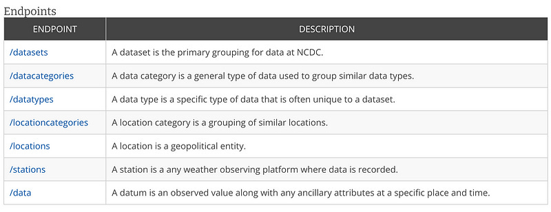
I began investigating the /data endpoint, and below you can find the additional parameters that can be used during a GET request to retrieve the data.
My goal was to retrieve historical temperature data for specific dates and locations while also enabling pagination for better data handling.
To achieve this, three essential parameters were necessary:
- datasetid
- startdate
- enddate
In my first post, I got the required datasetid, which is GHCND for the Daily Summaries dataset. The startdate and enddate should be provided in the format YYYY-MM-DD.
Next, I decided to investigate whether I could request only temperature data by using the datatype parameter. I retrieved the list of available data categories for the GHCND dataset, using the following API endpoint:
https://www.ncei.noaa.gov/cdo-web/api/v2/datacategories?datasetid=GHCND"
data_categories = cache.Cache("data-categories", func() string { return get_request("https://www.ncei.noaa.gov/cdo-web/api/v2/datacategories?datasetid=GHCND") })After making the API call, I received the following JSON response:
{
   "metadata":{
      "resultset":{
         "offset":1,
         "count":9,
         "limit":25
      }
   },
   "results":[
      {
         "name":"Evaporation",
         "id":"EVAP"
      },
      {
         "name":"Land",
         "id":"LAND"
      },
      {
         "name":"Precipitation",
         "id":"PRCP"
      },
      {
         "name":"Sky cover & clouds",
         "id":"SKY"
      },
      {
         "name":"Sunshine",
         "id":"SUN"
      },
      {
         "name":"Air Temperature",
         "id":"TEMP"
      },
      {
         "name":"Water",
         "id":"WATER"
      },
      {
         "name":"Wind",
         "id":"WIND"
      },
      {
         "name":"Weather Type",
         "id":"WXTYPE"
      }
   ]
}
It was obvious to me that the TEMP category was the most suitable choice for my needs. To get more insights, I made another API request to fetch the data types for this category using the following URL:
https://www.ncei.noaa.gov/cdo-web/api/v2/datatypes?datasetid=GHCND&datacategoryid=TEMP
data_types = cache.Cache("data-types", func() string { return get_request("https://www.ncei.noaa.gov/cdo-web/api/v2/datatypes?datasetid=GHCND&datacategoryid=TEMP") })The response contained a list of different data types related to temperature data:
{
   "metadata":{
      "resultset":{
         "offset":1,
         "count":8,
         "limit":136
      }
   },
   "results":[
      {
         "mindate":"1863-05-04",
         "maxdate":"2023-07-08",
         "name":"Number of days included in the multiday minimum temperature (MDTN)",
         "datacoverage":1,
         "id":"DATN"
      },
      {
         "mindate":"1863-05-04",
         "maxdate":"2023-07-07",
         "name":"Number of days included in the multiday maximum temperature (MDTX)",
         "datacoverage":1,
         "id":"DATX"
      },
      {
         "mindate":"1863-05-04",
         "maxdate":"2023-07-08",
         "name":"Multiday minimum temperature (use with DATN)",
         "datacoverage":1,
         "id":"MDTN"
      },
      {
         "mindate":"1863-05-04",
         "maxdate":"2023-07-07",
         "name":"Multiday maximum temperature (use with DATX)",
         "datacoverage":1,
         "id":"MDTX"
      },
      {
         "mindate":"1874-10-13",
         "maxdate":"2023-07-12",
         "name":"Average Temperature.",
         "datacoverage":1,
         "id":"TAVG"
      },
      {
         "mindate":"1763-01-01",
         "maxdate":"2023-07-12",
         "name":"Maximum temperature",
         "datacoverage":1,
         "id":"TMAX"
      },
      {
         "mindate":"1763-01-01",
         "maxdate":"2023-07-12",
         "name":"Minimum temperature",
         "datacoverage":1,
         "id":"TMIN"
      },
      {
         "mindate":"1876-11-27",
         "maxdate":"2023-07-12",
         "name":"Temperature at the time of observation",
         "datacoverage":1,
         "id":"TOBS"
      }
   ]
}
After having the data types I needed: TAVG, TMAX, and TMIN, I proceeded to construct the request URL for fetching the data itself:
Additionally, I had the option to filter the data based on its location. To explore the available location categories for the locationid parameter, I made the following request:
https://www.ncei.noaa.gov/cdo-web/api/v2/locationcategories
location_categories = cache.Cache("location_categories", func() string { return get_request("https://www.ncei.noaa.gov/cdo-web/api/v2/locationcategories") })The response listed various location categories that could be used with the locationid parameter to filter data for specific cities, countries, and more.
{
   "metadata":{
      "resultset":{
         "offset":1,
         "count":12,
         "limit":25
      }
   },
   "results":[
      {
         "name":"City",
         "id":"CITY"
      },
      {
         "name":"Climate Division",
         "id":"CLIM_DIV"
      },
      {
         "name":"Climate Region",
         "id":"CLIM_REG"
      },
      {
         "name":"Country",
         "id":"CNTRY"
      },
      {
         "name":"County",
         "id":"CNTY"
      },
      {
         "name":"Hydrologic Accounting Unit",
         "id":"HYD_ACC"
      },
      {
         "name":"Hydrologic Cataloging Unit",
         "id":"HYD_CAT"
      },
      {
         "name":"Hydrologic Region",
         "id":"HYD_REG"
      },
      {
         "name":"Hydrologic Subregion",
         "id":"HYD_SUB"
      },
      {
         "name":"State",
         "id":"ST"
      },
      {
         "name":"US Territory",
         "id":"US_TERR"
      },
      {
         "name":"Zip Code",
         "id":"ZIP"
      }
   ]
}
As an example, to obtain a list of all cities, sorted by city names in descending order, I used the following url:
https://www.ncei.noaa.gov/cdo-web/api/v2/locations?locationcategoryid=CITY&sortfield=name&sortorder=desc&limit=100
cities_locations = cache.Cache("locations-cit1y", func() string { return get_request("https://www.ncei.noaa.gov/cdo-web/api/v2/locations?locationcategoryid=CITY&sortfield=name&sortorder=desc&limit=100") })From the JSON that I got that time, it was evident that there were a total of 1989 cities, and each city entry included information about the minimum and maximum dates of available data, as well as the city ID.
{
   "metadata":{
      "resultset":{
         "offset":1,
         "count":1989,
         "limit":100
      }
   },
   "results":[
      {
         "mindate":"1892-08-01",
         "maxdate":"2023-05-31",
         "name":"Zwolle, NL",
         "datacoverage":1,
         "id":"CITY:NL000012"
      },
      {
         "mindate":"1901-01-01",
         "maxdate":"2023-07-11",
         "name":"Zurich, SZ",
         "datacoverage":1,
         "id":"CITY:SZ000007"
      },
      {
         "mindate":"1957-07-01",
         "maxdate":"2023-07-11",
         "name":"Zonguldak, TU",
         "datacoverage":1,
         "id":"CITY:TU000057"
      },
      {
         "mindate":"1906-01-01",
         "maxdate":"2023-07-11",
         "name":"Zinder, NG",
         "datacoverage":0.9025,
         "id":"CITY:NG000004"
      },
...
The same approach can be applied for all location types by setting the “locationcategoryid” parameter to the appropriate location ID. Just another example, ZIP codes:
zip_code_locations = cache.Cache("zip-code-locations", func() string { return get_request("https://www.ncei.noaa.gov/cdo-web/api/v2/locations?locationcategoryid=ZIP&sortfield=name&sortorder=desc&limit=100") })Alright, it’s time to delve into real data! For this example, I selected Zurich with the location ID “CITY:SZ000007”. I then made a request for the GHCND report for May 1, 2022, with temperature units in metric.
Here’s the API request URL:
https://www.ncei.noaa.gov/cdo-web/api/v2/data?datasetid=GHCND&locationid=CITY:SZ000007&startdate=2022-05-01&enddate=2022-05-01&units=metric
data_city = cache.Cache("data-daily-city-sample", func() string { return get_request("https://www.ncei.noaa.gov/cdo-web/api/v2/data?datasetid=GHCND&locationid=CITY:SZ000007&startdate=2022-05-01&enddate=2022-05-01&units=metric") })After sending the request, I obtained the following JSON response:
{
   "metadata":{
      "resultset":{
         "offset":1,
         "count":3,
         "limit":25
      }
   },
   "results":[
      {
         "date":"2022-05-01T00:00:00",
         "datatype":"TAVG",
         "station":"GHCND:SZ000003700",
         "attributes":"H,,S,",
         "value":10.5
      },
      {
         "date":"2022-05-01T00:00:00",
         "datatype":"TMAX",
         "station":"GHCND:SZ000003700",
         "attributes":",,E,",
         "value":16.2
      },
      {
         "date":"2022-05-01T00:00:00",
         "datatype":"TMIN",
         "station":"GHCND:SZ000003700",
         "attributes":",,E,",
         "value":6.5
      }
   ]
}
As you might notice, the average temperature in Zurich on May 1, 2022, was 10.5 degrees Celsius and there was only one station in Zurich with the ID “GHCND:SZ000003700” which appears to be the source of this recorded data.
So I read here:
Stations are where the data comes from (for most datasets) and can be considered the smallest granual of location data
This means that with CDO API we have the flexibility to request data not just by the location ID but also by using the station ID as a parameter. So, for our analysis, we can access data from specific stations as well.
To get a list of all the available station IDs, I used the /stations endpoint. Here is the API request URL for that:
https://www.ncei.noaa.gov/cdo-web/api/v2/stations?datasetid=GHCND&limit=100
stations = cache.Cache("stations-GHCND", func() string { return get_request("https://www.ncei.noaa.gov/cdo-web/api/v2/stations?datasetid=GHCND&limit=100") })Upon examining the data fetched from the /stations endpoint, I discovered a list of 124,946 stations available in total. For each station, valuable information such as its coordinates (latitude and longitude) and the date range of existing data was provided.
Here’s a sample of the data I got:
{
   "metadata":{
      "resultset":{
         "offset":1,
         "count":124946,
         "limit":100
      }
   },
   "results":[
      {
         "elevation":10.1,
         "mindate":"1949-01-01",
         "maxdate":"1949-08-14",
         "latitude":17.11667,
         "name":"ST JOHNS COOLIDGE FIELD, AC",
         "datacoverage":1,
         "id":"GHCND:ACW00011604",
         "elevationUnit":"METERS",
         "longitude":-61.78333
      },
      {
         "elevation":19.2,
         "mindate":"1957-09-01",
         "maxdate":"1970-02-13",
         "latitude":17.13333,
         "name":"ST JOHNS, AC",
         "datacoverage":0.9723,
         "id":"GHCND:ACW00011647",
         "elevationUnit":"METERS",
         "longitude":-61.78333
      },
If I used the Zurich station ID in the request instead of the Zurich location ID, I would receive the same JSON, as there was only one station in Zurich at that date.
data_station = cache.Cache("data-daily-sample", func() string { return get_request("https://www.ncei.noaa.gov/cdo-web/api/v2/data?datasetid=GHCND&stationid=GHCND:SZ000003700&startdate=2022-05-01&enddate=2022-05-01&datatypeid=TMAX,TMIN,TAVG&units=metric") })Great! With the available data from various stations worldwide, I can retrieve average, minimum, and maximum temperatures for each location.
An important point to note is that we can use parameters limit and offset in the request URL, which enable us to implement pagination and make our data retrieval more manageable.
To ensure we’re all on the same page, I lazily asked ChatGPT for a concise explanation of what pagination means in this context.
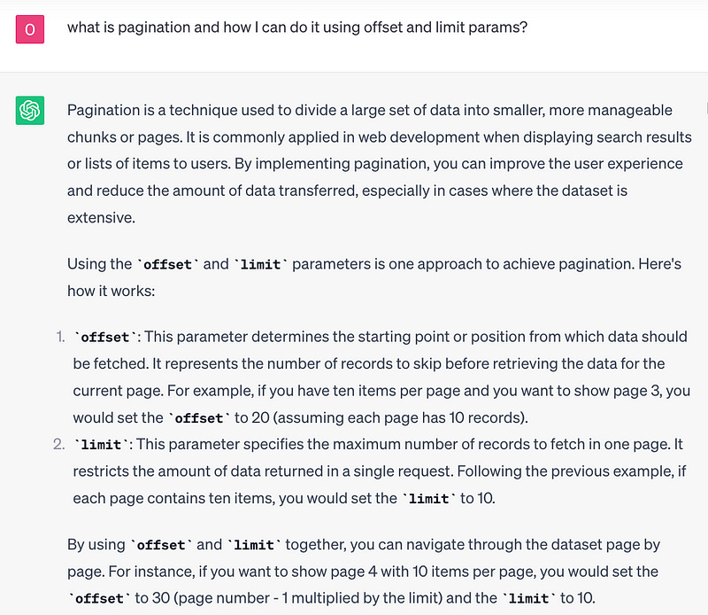
Thank you, ChatGPT for such a great explanation.
CDO Documentation
After diving into the CDO API and exploring the available data, I realized that finding some documentation on CDO itself would be super helpful.

First of all, I found a useful online search tool that allows to request historical datasets by applying filters and specifying locations.
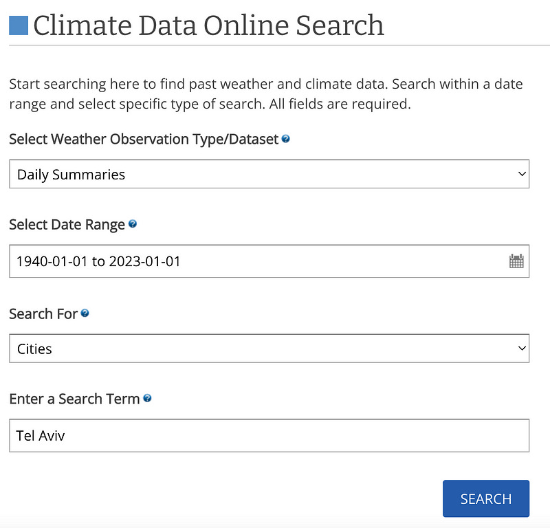
You can review the data by applying chosen filters. For instance, let’s take a look at the records available for 4 stations during a specific period in Tel Aviv.
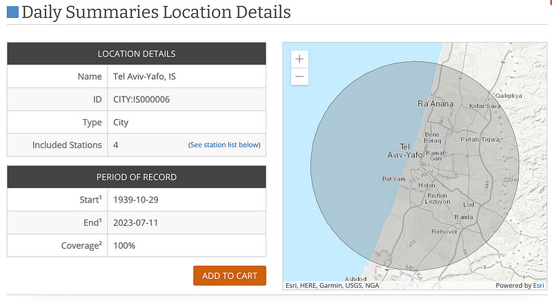
After selecting the data, you can also choose the output format, which includes options like CSV.
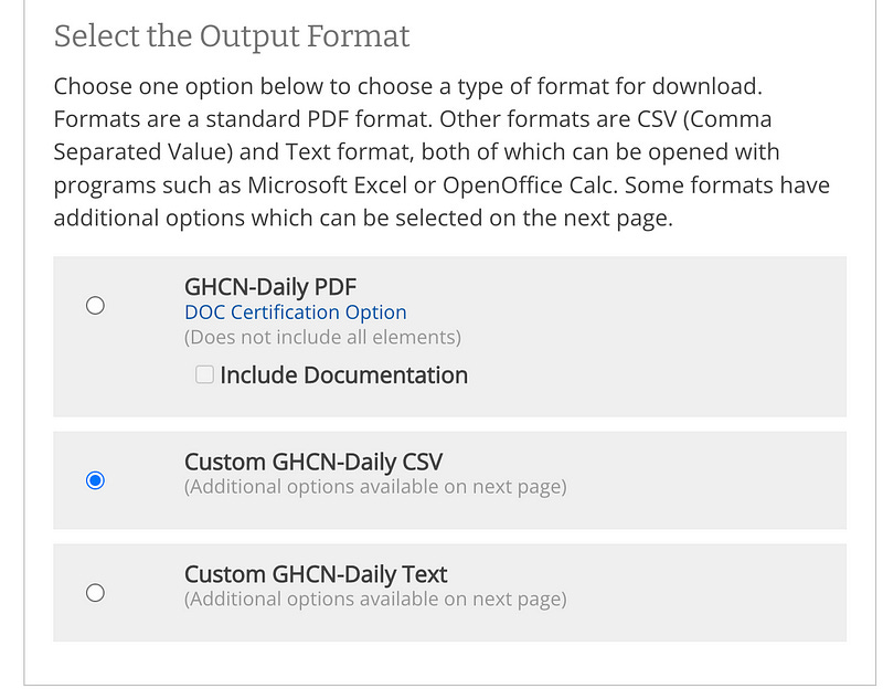
After that, you can select additional station details and data flags if needed.
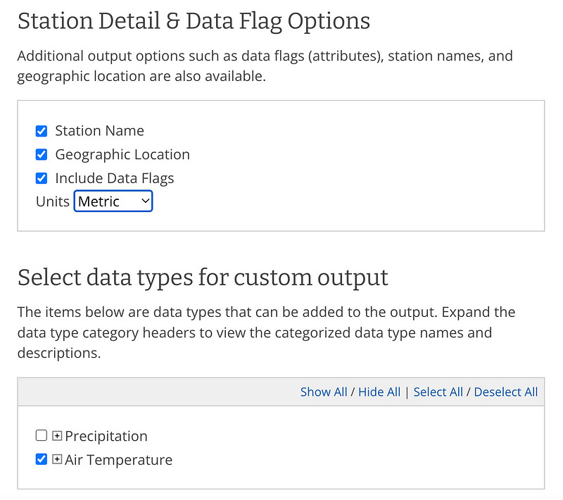
Later, they will ask for your email, and you’ll need to wait until they send you the report.
Meanwhile, I discovered that it’s also possible to download the entire historical archive, which is around 7Gb in size. However, I didn’t have enough space on my laptop to unpack it, as it required more than 150Gb. Another useful thing I found was the documentation section with a list of available stations and a description of the GHCN dataset. Based on the documentation, the report we requested:
Custom GHCN-Daily CSV- Output files contain .csv extension and optimized for spreadsheet usage (i.e. delimited file). Besides unit preference, user is also given the choice whether to include flags, station name or geographic location in data request. The user can define which of the elements listed in Table 4 (below) to include in the data request.
Finally, I got my CSV file with historical GHCND data for Tel Aviv. Now, let’s take a look at what’s inside. Also you can find this file in my repository.
The result:
"STATION","NAME","LATITUDE","LONGITUDE","ELEVATION","DATE","TAVG","TMAX","TMIN"
"IS000002011","TEL AVIV READING, IS","32.1","34.7831","3.0","1940-01-01",,,
"IS000002011","TEL AVIV READING, IS","32.1","34.7831","3.0","1940-01-02",,,
According to the CDO document, the data in the CSV file contains the following information:
- STATION (17 characters): The station identification code.
- STATION_NAME (max 50 characters): The name of the station, usually the city or airport name (optional field).
- GEOGRAPHIC_LOCATION (31 characters): The latitude (decimal degrees) with northern hemisphere values > 0 and southern hemisphere values 0, along with the elevation above mean sea level (tenths of meters) (optional field).
- DATE: The year of the record (4 digits) followed by the month (2 digits) and day (2 digits).
The additional values in the file are as follows:
- TMAX = Maximum temperature
- TMIN = Minimum temperature
- TAVG = Average temperature of hourly values
With this data, we can proceed with further investigation and think about how to visualize climate change.
Understanding the Visualization Needs for Climate Change
So, I now have access to historical temperature data that I downloaded from Climate Data Online Search. I can also schedule updates for this data using API endpoints. What’s next?
Before we continue doing the fancy stuff, let’s talk about the Climate Change Visualizer. What do people expect from such a product?
Well, people would expect straightforward and easy-to-read graphs that evidently display temperature trends and patterns over the years. These graphs can effectively explain what’s going on with the world’s climate. In essence, I would like to visualize how the climate has been changing over time in a clear and informative way.
For this reason, I decided to ask ChatGPT for some guidance.
So I’m creating Climate Change Visualizer as a pet project on Go, I loaded historical data from 1940 till now from GHCNd public set. I can get countries, cities, stations and “LATITUDE”,”LONGITUDE”,”ELEVATION”,”DATE”,”TAVG”,”TMAX”,”TMIN” for station. I would like to get your ideas on what visualization I can use here to show how climate changed. What graphs, maps?
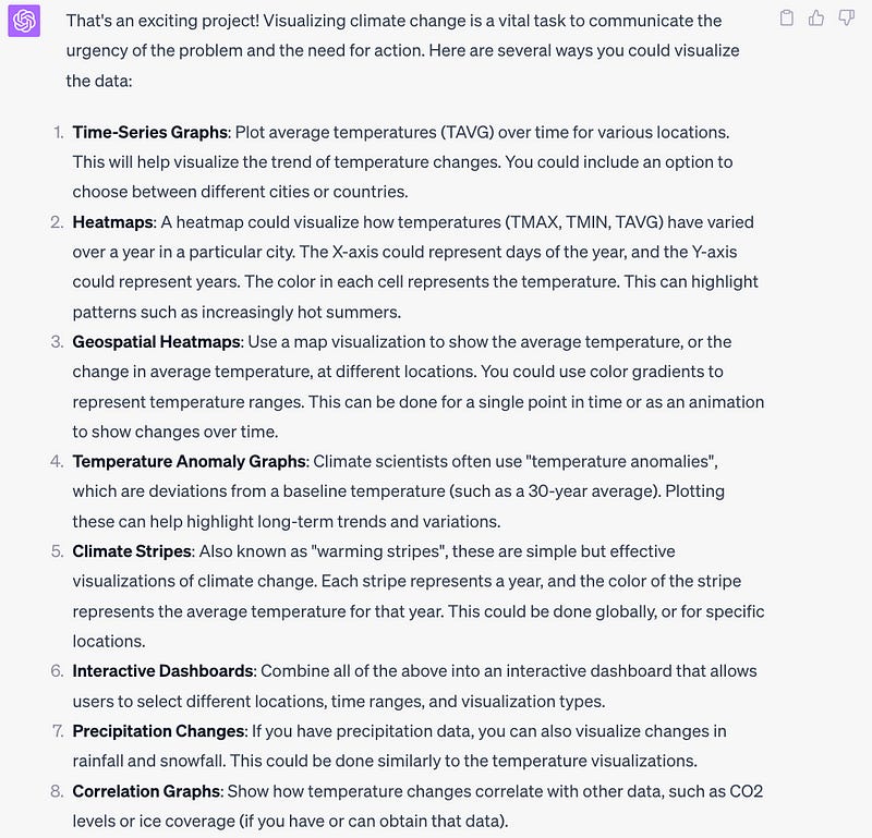
Quite a list. I didn’t want to overcomplicate it with additional data, except for average, minimal, and maximum temperature. Additionally, map visualization sounded like a longer project that wasn’t planned at this stage. Therefore, I narrowed down my choices to 1, 2, 4, and 5.
Let’s review them.
- Time-series graphs. Time-series graphs show data points plotted over time, where the x-axis represents chronological order and the y-axis displays the corresponding values. While they are a nice option, they may not offer the level of visual impact I’m aiming for. Instead, I believe a scatter plot that illustrates how the minimum and maximum temperatures change throughout years would be more suitable. Each dot on the scatter plot represents a specific year, with the x-axis indicating the average minimum temperature and the y-axis representing the average maximum temperature. The scatter plot’s visual arrangement will allow me to easily detect shifts in temperature distributions. The use of different colors for the dots further aids in identifying the years, making it simpler to spot significant changes in climate conditions.
- Heatmap. In this type of graph, each cell represents the temperature for a specific year and month combination. The colors of the cells correspond to the temperature values, with warmer colors indicating higher temperatures and cooler colors representing lower temperatures. Using this visualization, I can easily identify average temperature patterns throughout the years.
- Temperature Anomaly Graph. This graph displays the deviation of temperatures from a long-term average. Positive anomalies are shown above the baseline, indicating temperatures above the average, while negative anomalies are displayed below the baseline, representing temperatures below the average. With this visualization, I can easily identify patterns and trends in temperature variations, which will help me detect periods of warming or cooling over time.
- Climate Change Stripes. This graph creatively displays the temperature data using colored stripes to represent each year’s average temperature. Each stripe corresponds to a year, and the color intensity reflects the temperature value for that year. Warmer years are represented with warmer colors, and cooler years with cooler colors. With this visualization, I can quickly grasp temperature trends over the years and identify any long-term changes or anomalies.
After delving into various graph types like scatter plots, heatmaps, climate change stripes, and temperature anomaly graphs, I now have a set of visualization tools to comprehend climate change data. These graphs provide insights into temperature trends, seasonal variations, and anomalies, offering valuable information. With these visualizations, I’m excited to explore Golang’s capabilities in the next chapter. I hope that Golang possesses the necessary tools to handle graphing tasks effectively.
Conclusion
In this part of my Golang journey, I explored climate data through the Daily Summaries dataset. My focus was on understanding the available data and how to filter it using the CDO API. I learned about different data formats and endpoints, gaining insights into the possibilities for retrieving climate information.
During my exploration, I came across various graphs like scatter plots, heatmaps, climate change stripes, and temperature anomaly graphs. These visualizations will help us understand temperature trends and seasonal changes in the next chapters.
Stay tuned for more progress and discoveries in the next part of “The Golang Saga: A Coder’s Journey There and Back Again.”
Previous articles:

Next articles:


